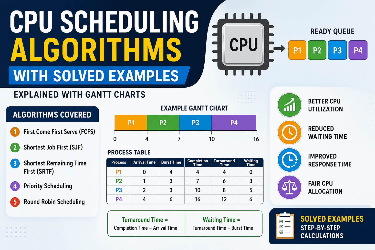
CPU Scheduling Algorithms with Solved Examples
Understanding CPU Scheduling Algorithms with Solved Examples is useful for computer science students, freshers, programmers, and candidates preparing for technical interviews. In this guide, we will discuss the major CPU scheduling methods, their formulas, advantages, disadvantages, and step-by-step examples.
What Is CPU Scheduling?
CPU scheduling is the process used by an operating system to select one process from the ready queue and assign the CPU to that process. The main purpose of scheduling is to use the processor efficiently while reducing waiting time, turnaround time, and response time.
When a process enters the system, it may wait in the ready queue until the CPU becomes available. The CPU scheduler checks the available processes and selects one according to a scheduling algorithm.
Important Terms Used in CPU Scheduling
Before studying the different algorithms, you should understand the following terms:
- Arrival Time: The time at which a process enters the ready queue.
- Burst Time: The total CPU execution time required by a process.
- Completion Time: The time at which the execution of a process is completed.
- Turnaround Time: The total time spent by a process in the system.
- Waiting Time: The total time a process waits in the ready queue.
- Response Time: The time between process arrival and its first CPU allocation.
Turnaround Time Formula:
Turnaround Time = Completion Time − Arrival Time
Waiting Time Formula:
Waiting Time = Turnaround Time − Burst Time
Types of CPU Scheduling Algorithms
The most commonly used CPU scheduling algorithms are:
- First Come First Serve
- Shortest Job First
- Shortest Remaining Time First
- Priority Scheduling
- Round Robin Scheduling
- Multilevel Queue Scheduling
1. First Come First Serve Scheduling
First Come First Serve, also known as FCFS, is the simplest CPU scheduling algorithm. The process that arrives first gets the CPU first. It works like a normal queue where the first person entering the queue is served before others.
FCFS is a non-preemptive algorithm. Once a process starts execution, it continues until its CPU burst is completed.
FCFS Solved Example
| Process | Arrival Time | Burst Time |
|---|---|---|
| P1 | 0 | 5 |
| P2 | 1 | 3 |
| P3 | 2 | 2 |
The processes will execute in the order P1, P2, and P3.
Gantt Chart:
P1: 0–5 | P2: 5–8 | P3: 8–10
| Process | Completion Time | Turnaround Time | Waiting Time |
|---|---|---|---|
| P1 | 5 | 5 − 0 = 5 | 5 − 5 = 0 |
| P2 | 8 | 8 − 1 = 7 | 7 − 3 = 4 |
| P3 | 10 | 10 − 2 = 8 | 8 − 2 = 6 |
Average Waiting Time = (0 + 4 + 6) ÷ 3 = 3.33 units
Advantages of FCFS
- Easy to understand and implement.
- Every process gets a chance to execute.
- No complex decision-making is required.
Disadvantages of FCFS
- A long process can delay all shorter processes.
- It may produce a high average waiting time.
- It suffers from the convoy effect.
2. Shortest Job First Scheduling
Shortest Job First, or SJF, selects the process with the shortest burst time. It can significantly reduce the average waiting time when the burst time of each process is known.
The non-preemptive version allows a selected process to finish completely before another process is chosen.
SJF Solved Example
| Process | Arrival Time | Burst Time |
|---|---|---|
| P1 | 0 | 6 |
| P2 | 0 | 2 |
| P3 | 0 | 4 |
All processes arrive at the same time. Therefore, the process with the lowest burst time will run first.
Execution Order: P2, P3, P1
Gantt Chart:
P2: 0–2 | P3: 2–6 | P1: 6–12
| Process | Completion Time | Turnaround Time | Waiting Time |
|---|---|---|---|
| P2 | 2 | 2 | 2 − 2 = 0 |
| P3 | 6 | 6 | 6 − 4 = 2 |
| P1 | 12 | 12 | 12 − 6 = 6 |
Average Waiting Time = (0 + 2 + 6) ÷ 3 = 2.67 units
Advantages of SJF
- It generally provides a low average waiting time.
- Short processes are completed quickly.
- It is suitable for batch-processing systems.
Disadvantages of SJF
- The exact burst time is difficult to predict.
- Long processes may experience starvation.
- It is not ideal for interactive systems.
3. Shortest Remaining Time First
Shortest Remaining Time First, or SRTF, is the preemptive version of SJF. In this method, the operating system always executes the process with the lowest remaining burst time.
When a new process arrives with a shorter burst time than the remaining time of the currently running process, the current process is interrupted.
SRTF Solved Example
| Process | Arrival Time | Burst Time |
|---|---|---|
| P1 | 0 | 7 |
| P2 | 2 | 4 |
| P3 | 4 | 1 |
P1 starts at time 0. At time 2, P2 arrives with a shorter burst time, so P1 is paused. At time 4, P3 arrives with only one unit of burst time, so it executes immediately.
Gantt Chart:
P1: 0–2 | P2: 2–4 | P3: 4–5 | P2: 5–7 | P1: 7–12
The completion times are P3 = 5, P2 = 7, and P1 = 12.
4. Priority Scheduling
In Priority Scheduling, every process is assigned a priority number. The CPU is allocated to the process with the highest priority. Depending on the operating system, a smaller priority number may represent a higher priority.
Priority Scheduling Solved Example
| Process | Burst Time | Priority |
|---|---|---|
| P1 | 5 | 3 |
| P2 | 3 | 1 |
| P3 | 4 | 2 |
Assume that a smaller number means a higher priority. Therefore, the execution order will be P2, P3, and P1.
Gantt Chart:
P2: 0–3 | P3: 3–7 | P1: 7–12
Waiting time of P2 = 0
Waiting time of P3 = 3
Waiting time of P1 = 7
Average Waiting Time = (0 + 3 + 7) ÷ 3 = 3.33 units
The biggest problem with Priority Scheduling is starvation. A low-priority process may wait for a very long time. This issue can be reduced through aging, where the priority of a waiting process gradually increases.
5. Round Robin Scheduling
Round Robin is a preemptive scheduling algorithm commonly used in time-sharing systems. Each process receives a fixed amount of CPU time called a time quantum.
If a process does not finish within the given time quantum, it is moved to the end of the ready queue.
Round Robin Solved Example
| Process | Burst Time |
|---|---|
| P1 | 5 |
| P2 | 4 |
| P3 | 2 |
Assume that the time quantum is 2 units.
Gantt Chart:
P1: 0–2 | P2: 2–4 | P3: 4–6 | P1: 6–8 | P2: 8–10 | P1: 10–11
Completion time of P3 = 6
Completion time of P2 = 10
Completion time of P1 = 11
Since all processes arrive at time 0:
Waiting Time of P1 = 11 − 5 = 6
Waiting Time of P2 = 10 − 4 = 6
Waiting Time of P3 = 6 − 2 = 4
Average Waiting Time = (6 + 6 + 4) ÷ 3 = 5.33 units
Advantages of Round Robin
- Every process receives a fair share of CPU time.
- It provides a better response time for interactive tasks.
- It prevents a single process from using the CPU for too long.
Disadvantages of Round Robin
- A very small time quantum increases context switching.
- A large time quantum makes it similar to FCFS.
- Performance depends heavily on the selected time quantum.
Comparison of CPU Scheduling Algorithms
| Algorithm | Type | Main Selection Rule | Major Problem |
|---|---|---|---|
| FCFS | Non-preemptive | First arrival | Convoy effect |
| SJF | Non-preemptive | Shortest burst time | Starvation |
| SRTF | Preemptive | Shortest remaining time | Frequent switching |
| Priority | Both | Highest priority | Starvation |
| Round Robin | Preemptive | Fixed time quantum | Context-switch overhead |
Which CPU Scheduling Algorithm Is Best?
There is no single scheduling algorithm that is best for every operating system. FCFS is simple but may increase waiting time. SJF offers a low average waiting time but requires burst-time prediction. Priority Scheduling is useful for important tasks, while Round Robin is better for interactive and time-sharing environments.
The final choice depends on system requirements, response-time expectations, process types, and available resources.
Frequently Asked Questions
What is the main purpose of CPU scheduling?
The main purpose is to select the next process for execution, improve CPU utilization, and reduce waiting and turnaround time.
Which algorithm gives the minimum average waiting time?
Shortest Job First generally provides the minimum average waiting time when accurate burst times are available.
Is Round Robin preemptive?
Yes. Round Robin is a preemptive algorithm because a process is interrupted after its assigned time quantum expires.
What is starvation in CPU scheduling?
Starvation occurs when a process waits indefinitely because other processes continue receiving CPU time before it.
Conclusion
CPU scheduling plays a major role in the performance of an operating system. Algorithms such as FCFS, SJF, SRTF, Priority Scheduling, and Round Robin use different rules to select processes from the ready queue.
By studying CPU Scheduling Algorithms with Solved Examples, you can understand how completion time, turnaround time, waiting time, and process order are calculated. These concepts are frequently asked in operating-system examinations, placement tests, and technical interviews. Practising more Gantt chart problems is the best way to master CPU scheduling calculations.